In this blog post, we’ll explore how to make use of SARIMAX, a powerful statistical method, in conjunction with machine learning techniques for time series forecasting using Python within the mobility industry.
With the introduction of machine learning, traditional statistical methods have been enhanced to deliver more accurate and robust predictions.
In ride-hailing, predicting customer volumes is essential for optimising operations, managing resources efficiently, and enhancing customer experience. This can be achieved with time series forecasting techniques like SARIMAX.
Time series forecasting techniques like SARIMAX can play a crucial role in this regard.
We will demonstrate how we can apply SARIMAX to predict customer volumes in the mobility sector.
What is SARIMAX?
Seasonal Autoregressive Integrated Moving Average with Exogenous Regressors (SARIMAX) is a statistical method commonly used for time series analysis and forecasting.
It extends the ARIMA model by incorporating additional parameters for seasonal variations and exogenous variables.
SARIMAX models are widely used in industries such as finance, economics, and healthcare for predicting future values based on historical data patterns.
We also use it within the mobility industry.
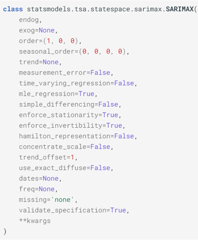
As can be seen in the below snapshot of possible inputs for this statistical method, the Python package has a diverse number of possible variables that the analyst can use to personalise the tool with.
The ones most typically amended with company-specific values are ‘order’ and ‘seasonal order’ and rest are commonly left with their default values as described here.
Mathematical Formulation
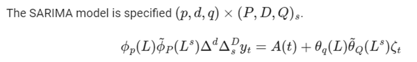
For the mathematically minded, this is how the method is defined using three sets of parameters.
The three sets of parameters:
- Seasonal Parameters (p, d, q, P, D, Q, s):
- p: Autoregressive order for the seasonal component.
- d: Degree of differencing for the seasonal component.
- q: Moving average order for the seasonal component.
- P: Seasonal autoregressive order.
- D: Degree of differencing for the seasonal component.
- Q: Seasonal moving average order.
- s: Seasonal period (e.g., 24 for hourly data, 7 for weekly data, 12 for monthly data and 4 for quarterly data)
- Non-seasonal Parameters (p, d, q):
- p: Autoregressive order for the non-seasonal component.
- d: Degree of differencing for the non-seasonal component.
- q: Moving average order for the non-seasonal component.
- Exogenous Variables (X):
- Additional variables that are incorporated into the model to capture their influence on the time series.
In ‘English’
- The Seasonal Component in SARIMAX accounts for seasonal patterns in the time series data. Seasonality refers to repeating patterns that occur at regular intervals, such as daily, weekly, or yearly cycles. By incorporating seasonal parameters, SARIMAX can capture and model these patterns effectively.
- The Autoregressive (AR) Component of The autoregressive component of SARIMAX models the relationship between an observation and a number of lagged observations (i.e., past values of the time series). This component captures the dependence of the current value on its previous values.
- The Integrated (I) Component: The integrated component of SARIMAX accounts for non-stationarity in the time series data by differencing. Non-stationarity refers to the presence of trends or irregular patterns that change over time. By differencing the data, SARIMAX transforms it into a stationary series, making it suitable for modelling.
- The Moving Average (MA) Component: The moving average component of SARIMAX models the dependency between an observation and a residual error from a moving average model applied to lagged observations. This component helps capture short-term fluctuations and noise in the data.
- The Exogenous Variables (X) in SARIMAX allows for the inclusion of exogenous variables, which are external factors that may influence the time series but are not part of the time series itself. These variables could be economic indicators, weather conditions, or any other relevant factors that affect the phenomenon being studied.
Workflow of SARIMAX Modelling
- Data Collection and Preparation:
One must first gather historical data on customer volumes from the company’s database or other such relevant sources. This data could include metrics such as the number of ride requests or bookings per hour/day. This data must then be pre-processed by handling missing values, removing outliers, and converting timestamps to appropriate datetime objects.
- Exploratory Data Analysis (EDA):
One must then conduct exploratory data analysis to understand any underlying patterns or trends in customer volumes. The time series data is then visualised using line plots, histograms, and seasonal decomposition to identify seasonality, trends, and any anomalies which are to be used in the next stage.
- Model Building:
The Machine Learning (ML) portion of the process starts here by splitting the dataset into training and testing sets, ensuring that the temporal order is maintained. A SARIMAX model is fit to the training data, specifying the appropriate parameters such as order and seasonal order based on the identified patterns in the data in the previous step. One may also include exogenous variables such as weather conditions, holidays, or events that may influence customer volumes at this stage.
- Model Evaluation:
The performance of the SARIMAX model is then evaluated using metrics such as Mean Absolute Error (MAE), Mean Squared Error (MSE), and Root Mean Squared Error (RMSE) on the testing set. The forecasted customer volumes are compared with the actual values to assess the accuracy of the model.
- Forecasting:
The trained SARIMAX model is then used to generate forecasts for future time periods, capturing variations in customer volumes. The forecasted customer volumes are visualised along with prediction intervals to provide insights into the uncertainty associated with the predictions.
Conclusion
Predicting important metrics as accurately as possible is vital for making data-driven decisions within businesses, particularly those within the mobility industry as it allows for the optimisation of operations and customer experience.
By making the most of the tools at hand, particularly packages like SARIMAX in Python for time series forecasting, ride-hailing companies such as eCabs can try to anticipate fluctuations in demand and supply within such a volatile market.